from fastai.vision.all import *Lesson Video:
What is our goal today?
- Learn about the fastai framework through a vision application
- Create a neural network that can distinguish between 26 different breeds of animals
- Become familiar the different sublibraries of fastai
Let’s grab the library:
The fastai library is segmented between vision, text, tabular, and collab, spanning across each of these applications.
While this course is only focused on the first, by the end of these 7 weeks this understanding will easily be able to propagate into the other 3 applications.
Since this course will be on vision, we import the vision module:
Authors Note: This import * is an extremely bad practice in modern Python programming. This shouldn’t be done in production, and each lecture will have all of the “exact” imports for everything used as a reference to both see what you should do and understand where everything comes from
General Deep Learning Pipeline:
We’ll be focusing on a small subset of this pipeline:
Looking at Data
Since we’re focusing on only those 4 latter, this course will rely on other curated datasets for our analysis. For today’s problem we will attempt to identify between 12 species of cats and 25 species of dogs (37 in total). 7 years ago state-of-the-art was considered 59% error.
Today, this is now < 10.
What we will try and do is build a world-class image classifier using the fastai API and achieve this in less than 10 minutes.
First we need this dataset. fastai has a data class to do so, through something called untar_data.
If we call help on untar_data, we can see it’s documentation description:
help(untar_data)Help on function untar_data in module fastai.data.external:
untar_data(url: 'str', archive: 'Path' = None, data: 'Path' = None, c_key: 'str' = 'data', force_download: 'bool' = False, base: 'str' = '~/.fastai') -> 'Path'
Download `url` using `FastDownload.get`
The first thing you may notice is this doesn’t say much. To get a bit better of a description you can rely on a framework called nbdev (what fastai is built upon), which enables their special documentation-writing schema to appear when asking for more information:
untar_data
 untar_data (url:str, archive:pathlib.Path=None, data:pathlib.Path=None,
             c_key:str='data', force_download:bool=False,
             base:str='~/.fastai')
Download url using FastDownload.get
| Type | Default | Details | |
|---|---|---|---|
| url | str | File to download | |
| archive | Path | None | Optional override for Config’s archive key |
| data | Path | None | Optional override for Config’s data key |
| c_key | str | data | Key in Config where to extract file |
| force_download | bool | False | Setting to True will overwrite any existing copy of data |
| base | str | ~/.fastai | Directory containing config file and base of relative paths |
| Returns | Path | Path to extracted file(s) |
fastai has a few preset datasets stored in a set of URLs. For our problem this lives in PETS, which contains the Oxford Pets dataset. This dataset is designed around identifying cats and dogs by species
Let’s download the dataset
path = untar_data(URLs.PETS)And set our seed to ensure we have reproducability
fastai takes a different approach to reproducibility as it’s a research library. Subtle differences can be good to be aware of to learn behavioral changes in your code. However, in practice your testing suites needs to be reproducable. These should be mixed if the situation makes sense, to provide a better tested framework
set_seed(42)How is our data setup?
path.ls()[:3](#2) [Path('/home/zach_mueller_huggingface_co/.fastai/data/oxford-iiit-pet/annotations'),Path('/home/zach_mueller_huggingface_co/.fastai/data/oxford-iiit-pet/images')]Seperated between images and annotations
Annotations in this case isn’t actually relevant to our problem, we only care about the images folder
(path/'images').ls()[:3](#3) [Path('/home/zach_mueller_huggingface_co/.fastai/data/oxford-iiit-pet/images/beagle_32.jpg'),Path('/home/zach_mueller_huggingface_co/.fastai/data/oxford-iiit-pet/images/yorkshire_terrier_86.jpg'),Path('/home/zach_mueller_huggingface_co/.fastai/data/oxford-iiit-pet/images/staffordshire_bull_terrier_68.jpg')]The true labels exist as part of the filename.
You may also notice that sometimes I use creative abilities that may not exist in the typical Python library, such as this Path.ls() that was just used. We’ll talk more about this in detail in lesson 6 but for now just understand the fastai suite has an ability to expand existing implementations that can be useful in the right context
Let’s build a DataLoaders. First we’ll need the path to our data, some filenames, and the regex pattern to extract our labels:
path = untar_data(URLs.PETS)
fnames = get_image_files(path/'images')
pat = r'(.+)_\d+.jpg$'
Some basic transforms for getting all of our images the same size (item_tfms), and some augmentations and Normalization to be done on the GPU (batch_tfms)
This has to be done because images must be the same size before they can be pushed to the GPU and have these augmentations be applied
item_tfms = RandomResizedCrop(460, min_scale=0.75, ratio=(1.,1.))
batch_tfms = [*aug_transforms(size=224, max_warp=0), Normalize.from_stats(*imagenet_stats)]
bs=64
Presentation
Back to DataLoaders
dls = ImageDataLoaders.from_name_re(
    path, # The location of the data
    fnames, # A list of filenames
    pat, # A regex pattern to extract the labels
    item_tfms=item_tfms, # Transform augmentations to be applied per item
    batch_tfms=batch_tfms, # Transform augmentations to be applied per batch
    bs=bs # How many examples should be drawn each time
)
Least readable in some cases, but if your particular problem fits this niche mindset, it can be helpful
Let’s rebuild using the DataBlock API, which explains a bit more of the magic occurring
We’ll need to define what our input and outputs should be (An Image and a Category for classification), how to get our items, how to split our data, how to extract our labels, and our augmentation as before:
pets = DataBlock(blocks=(ImageBlock, CategoryBlock),
                 get_items=get_image_files,
                 splitter=RandomSplitter(),
                 get_y=RegexLabeller(pat = r'/([^/]+)_\d+.*'),
                 item_tfms=item_tfms,
                 batch_tfms=batch_tfms)
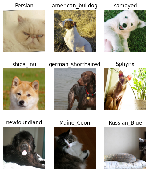
path_im = path/'images'dls = pets.dataloaders(path_im, bs=bs)We can take a look at a batch of our images using show_batch, pass in a maximum number of images to show, and how large we want to view them as
dls.show_batch(max_n=9, figsize=(6,7))
If we want to see how many classes we have, and the names of them we can simply call dls.vocab. The first is the number of classes, the second is the names of our classes. This is another special wrapper class, think of it as a special list of sorts, called L.
dls.vocab['Abyssinian', 'Bengal', 'Birman', 'Bombay', 'British_Shorthair', 'Egyptian_Mau', 'Maine_Coon', 'Persian', 'Ragdoll', 'Russian_Blue', 'Siamese', 'Sphynx', 'american_bulldog', 'american_pit_bull_terrier', 'basset_hound', 'beagle', 'boxer', 'chihuahua', 'english_cocker_spaniel', 'english_setter', 'german_shorthaired', 'great_pyrenees', 'havanese', 'japanese_chin', 'keeshond', 'leonberger', 'miniature_pinscher', 'newfoundland', 'pomeranian', 'pug', 'saint_bernard', 'samoyed', 'scottish_terrier', 'shiba_inu', 'staffordshire_bull_terrier', 'wheaten_terrier', 'yorkshire_terrier']In a more pythonic-fashion, the vocab also has an o2i (object to index) we can utilize instead
dls.vocab.o2i{'Abyssinian': 0,
'Bengal': 1,
'Birman': 2,
'Bombay': 3,
'British_Shorthair': 4,
'Egyptian_Mau': 5,
'Maine_Coon': 6,
'Persian': 7,
'Ragdoll': 8,
'Russian_Blue': 9,
'Siamese': 10,
'Sphynx': 11,
'american_bulldog': 12,
'american_pit_bull_terrier': 13,
'basset_hound': 14,
'beagle': 15,
'boxer': 16,
'chihuahua': 17,
'english_cocker_spaniel': 18,
'english_setter': 19,
'german_shorthaired': 20,
'great_pyrenees': 21,
'havanese': 22,
'japanese_chin': 23,
'keeshond': 24,
'leonberger': 25,
'miniature_pinscher': 26,
'newfoundland': 27,
'pomeranian': 28,
'pug': 29,
'saint_bernard': 30,
'samoyed': 31,
'scottish_terrier': 32,
'shiba_inu': 33,
'staffordshire_bull_terrier': 34,
'wheaten_terrier': 35,
'yorkshire_terrier': 36}Time to make and train a model!
We will be using a convolutional neural network backbone and a fully connected head with a single hidden layer as our classifier. Don’t worry if thats a bunch of nonsense for now. Right now, just know this: we are piggybacking off of a model to help us classify images into 37 categories.
Modern applied computer vision never starts from scratch. Instead we utilize a technique called transfer learning. Let someone else with much more compute than you build a state-of-the-art model, then piggyback off of this trained model for your own custom datasets.
In practice, this requires removing the last layer of the model and restructuring it to your problem.
Most commonly this comes in the form of a model trained on the ImageNet dataset (1,000 classes) and then downstreaming it to your own problem (37 classes).
To do so, we need 5 requirements:
DataLoaders- Some architecture
- A evaluation metric
- A loss function
- An optimizer
The fastai library will then wrap all of these items needed for training into the Learner. Oftentimes these don’t need to specified, as defaults are carefully picked out to have excellent performance right away.
Each module has their own _learner function that returns a Learner to facilitate training. Since we have a vision problem we utilize the vision_learner (convolutional). With these defaults, we also only need to pass in the DataLoaders, a model architecture, and the metric:
learn = vision_learner(dls, resnet34, metrics=error_rate)Downloading: "https://download.pytorch.org/models/resnet34-333f7ec4.pth" to /home/zach_mueller_huggingface_co/.cache/torch/hub/checkpoints/resnet34-333f7ec4.pthlearn = vision_learner(dls, resnet34, metrics=error_rate)Downloading: "https://download.pytorch.org/models/resnet34-333f7ec4.pth" to /home/zach_mueller_huggingface_co/.cache/torch/hub/checkpoints/resnet34-333f7ec4.pthresnet34This is a very common machine learning model to start with hosted by torchvision. Much like the example earlier it was trained on the ImageNet dataset of 1,000 classes
error_rateOur problem is graded by “amount wrong”, which takes the form of the error_rate metric
Each module has their own Learner:
vision:vision_learnertabular:tabular_learnertext:text_learnercollab:collab_learner
Some assumptions being made here:
- Loss function is assumed as classification, so
CrossEntropyFlatis used - Optimizer defaults to the AdamW optimizer, a commonly used optimizer that has been considered as a good starting place in the Deep Learning community for the past few years
With this now, we can train the model.
There’s a variety of “fit” functions fastai provides, each with their own set of hyperparameters to train a model. Generally fit_one_cycle (the One Cycle policy) or fit_flat_cos (Consine Annealing) are the best methods of training, which fastai simplifies to a simple one-line function:
learn.fit_one_cycle(4)| epoch | train_loss | valid_loss | error_rate | time |
|---|---|---|---|---|
| 0 | 1.939954 | 0.353235 | 0.109608 | 00:36 |
| 1 | 0.673132 | 0.257873 | 0.082544 | 00:36 |
| 2 | 0.374954 | 0.231789 | 0.076455 | 00:36 |
| 3 | 0.279564 | 0.224494 | 0.069689 | 00:36 |
Afterwards we can save the model weights:
learn.save('stage_1')Path('models/stage_1.pth')Analyzing how the model performed
With the model trained, the next step in the feedback loop is looking at where it messed up. What species did it have trouble differentiating between? So long as the misidentifications are not too bad, our model is actually working.
What counts as being “too bad” is never an exact science, often when working on problems a deep learning engineer should be paired with an expert in the respective problem field so that these analysis have the proper context
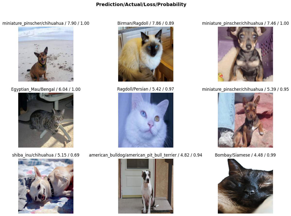
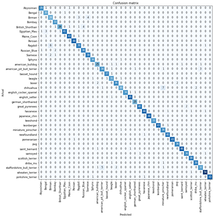
We can plot our losses and make a confusion matrix to visualize these through the ClassificationInterpretation interface:
interp = ClassificationInterpretation.from_learner(learn)plot_top_losses needs x number of images to examine, and a figure size.
interp.plot_top_losses(9, figsize=(15,10))
plot_confusion_matrix just needs a figure size. dpi adjusts the quality
interp.plot_confusion_matrix(figsize=(12,12), dpi=60)
We can also directly grab our most confused (A raw version of the confusion matrix), and pass in a threshold
interp.most_confused(min_val=3)[('chihuahua', 'miniature_pinscher', 7),
('Ragdoll', 'Birman', 6),
('staffordshire_bull_terrier', 'american_pit_bull_terrier', 5),
('Birman', 'Siamese', 4),
('British_Shorthair', 'Russian_Blue', 4),
('Birman', 'Ragdoll', 3),
('Egyptian_Mau', 'Bengal', 3),
('american_pit_bull_terrier', 'staffordshire_bull_terrier', 3)]Unfreezing our model, fine-tuning, and our learning rates
So, we have the model. Let’s fine tune it. First, we need to load our model back in.
learn.load('stage_1');Now we will unfreeze and train more
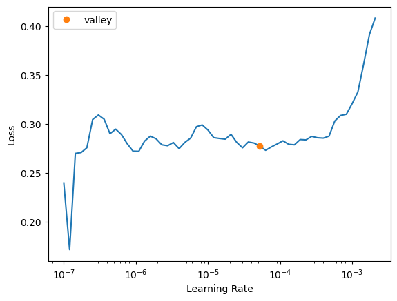
learn.unfreeze()Now when we unfreeze, we unfreeze all the layers. To find a proper new learning rate we can use the learning rate finder to help:
learn.lr_find()SuggestedLRs(valley=5.248074739938602e-05)
Alright so if we look here, we don’t start really spiking our losses until ~10^-2 so a good spot is between 1e-6 and 1e-4. We can pass this in as a maximum learning rate:
learn.fit_one_cycle(4, lr_max=slice(1e-6, 1e-4))| epoch | train_loss | valid_loss | error_rate | time |
|---|---|---|---|---|
| 0 | 0.257934 | 0.215489 | 0.071042 | 00:41 |
| 1 | 0.249958 | 0.203696 | 0.064276 | 00:40 |
| 2 | 0.211961 | 0.207521 | 0.067659 | 00:40 |
| 3 | 0.187639 | 0.202181 | 0.066982 | 00:40 |
We can see that picking a proper learning rate can help achieve a lower error rate and train a better model
learn.save('stage_2')Path('models/stage_2.pth')